tabpfn, meaning prior fitted networks for tabular data, is a deep-learning model. See:
- Transformers Can Do Bayesian Inference (arXiv, 2021)
- TabPFN: A Transformer That Solves Small Tabular Classification Problems in a Second (arXiv, 2022)
- Accurate predictions on small data with a tabular foundation model (Nature, 2025)
This R package is a wrapper of the Python library via reticulate. It has an idiomatic R syntax using standard S3 methods.
Installation
You can install the development version of tabpfn like so:
You’ll need a Python virtual environment to access the underlying library. After installing the R package, tabpfn will install the required Python bits when you first fit a model:
> library(tabpfn)
>
> predictors <- mtcars[, -1]
> outcome <- mtcars[, 1]
>
> # XY interface
> mod <- tab_pfn(predictors, outcome)
Downloading uv...Done!
Downloading cpython-3.12.12 (download) (15.9MiB)
 Downloading cpython-3.12.12 (download)
Downloading setuptools (1.1MiB)
Downloading scikit-learn (8.2MiB)
Downloading numpy (4.9MiB)

<downloading and installing more packages>

 Downloading llvmlite
 Downloading torch
Installed 58 packages in 350ms
> mod
tabpfn Regression Model

Training set
i 32 data points
i 10 predictors
Example
To fit a model:
set.seed(364)
reg_mod <- tab_pfn(mtcars[1:25, -1], mtcars$mpg[1:25])
reg_mod
#> TabPFN Regression Model
#> Training set
#> ℹ 25 data points
#> ℹ 10 predictors
In addition to the x/y interface shown above, there are also formula and recipes interfaces.
Prediction follows the usual S3 predict() method:
predict(reg_mod, mtcars[26:32, -1])
#> # A tibble: 7 × 1
#>   .pred
#>   <dbl>
#> 1  29.8
#> 2  25.6
#> 3  26.2
#> 4  16.5
#> 5  19.4
#> 6  14.7
#> 7  23.6
tabpfn follows the tidymodels prediction convention: a data frame is always returned with a standard set of column names.
For a classification model, the outcome should always be a factor vector. For example, using these data from the modeldata package:
library(modeldata)
#>
#> Attaching package: 'modeldata'
#> The following object is masked from 'package:datasets':
#>
#>     penguins
library(ggplot2)

two_cls_train <- parabolic[1:400,  ]
two_cls_val   <- parabolic[401:500,]
grid <- expand.grid(X1 = seq(-5.1, 5.0, length.out = 25),
                    X2 = seq(-5.5, 4.0, length.out = 25))

set.seed(3824)
cls_mod <- tab_pfn(class ~ ., data = two_cls_train)

grid_pred <- predict(cls_mod, grid)
grid_pred
#> # A tibble: 625 × 3
#>    .pred_Class1 .pred_Class2 .pred_class
#>           <dbl>        <dbl> <fct>
#>  1        0.988      0.0122  Class1
#>  2        0.992      0.00823 Class1
#>  3        0.993      0.00721 Class1
#>  4        0.993      0.00714 Class1
#>  5        0.991      0.00944 Class1
#>  6        0.982      0.0175  Class1
#>  7        0.965      0.0347  Class1
#>  8        0.922      0.0775  Class1
#>  9        0.799      0.201   Class1
#> 10        0.554      0.446   Class1
#> # ℹ 615 more rows
The fit looks fairly good when shown with out-of-sample data:
cbind(grid, grid_pred) |>
 ggplot(aes(X1, X2)) +
 geom_point(data = two_cls_val, aes(col = class, pch = class),
            alpha = 3 / 4, cex = 3) +
 geom_contour(aes(z = .pred_Class1), breaks = 1/ 2, col = "black", linewidth = 1) +
 coord_equal(ratio = 1)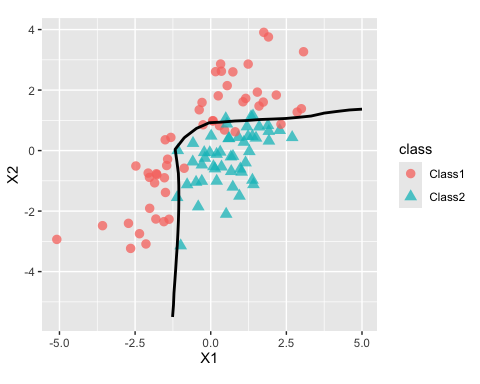
Code of Conduct
Please note that the tabpfn project is released with a Contributor Code of Conduct. By contributing to this project, you agree to abide by its terms.